---
title: "Building a Production-Grade LLM Inference Stack: Benchmarking vLLM, Ray Serve, and MoE Models"
author:
- "Vinay Pandya"
- "Yiran Xu"
date: "2026-04-25"
categories: [llm, inference, vllm, ray-serve, moe, benchmarking, deep-learning]
toc: true
toc-depth: 3
number-sections: true
highlight-style: github
code-fold: true
code-tools: true
execute:
eval: false
warning: false
message: false
---
```{python}
#| label: setup
#| include: false
import pandas as pd
import plotly.express as px
import plotly.graph_objects as go
from plotly.subplots import make_subplots
import numpy as np
# Set default plotly template
import plotly.io as pio
pio.templates.default = "plotly_white"
# Load all result CSVs
qwen_results = pd.read_csv("results/qwen_vllm_model_sharegpt_concurrency_20260411_131143.csv")
deepseek_disagg = pd.read_csv("results/deepseek_sharegpt_concurrency_20260411_132403.csv")
modal_lmcache = pd.read_csv("results/modal_vllm_lmcache_sharegpt_concurrency_20260408_141225.csv")
# Note: Add path for non-disaggregated DeepSeek results when available
```
## Introduction
Self-hosting Large Language Models (LLMs) has become increasingly important for organizations seeking to balance cost, latency, and data privacy. But choosing the right inference stack involves navigating a complex landscape of serving frameworks, model architectures, and infrastructure options.
In this post, I share hands-on benchmarking results from building a production-grade LLM inference platform. We'll compare:
- **Qwen2.5-7B** on Ray Serve + vLLM (production baseline)
- **DeepSeek-V2-Lite MoE** with and without disaggregated prefill
- **LLaMA 3.1-8B** with LMCache on Modal (serverless)
::: {.callout-tip}
## Key Takeaway
Infrastructure choices matter as much as model selection. The same MoE model showed **13x throughput difference** based solely on whether disaggregated prefill was enabled.
:::
## Architecture Overview
### The Full Stack
Our inference platform consists of multiple layers, each serving a specific purpose:
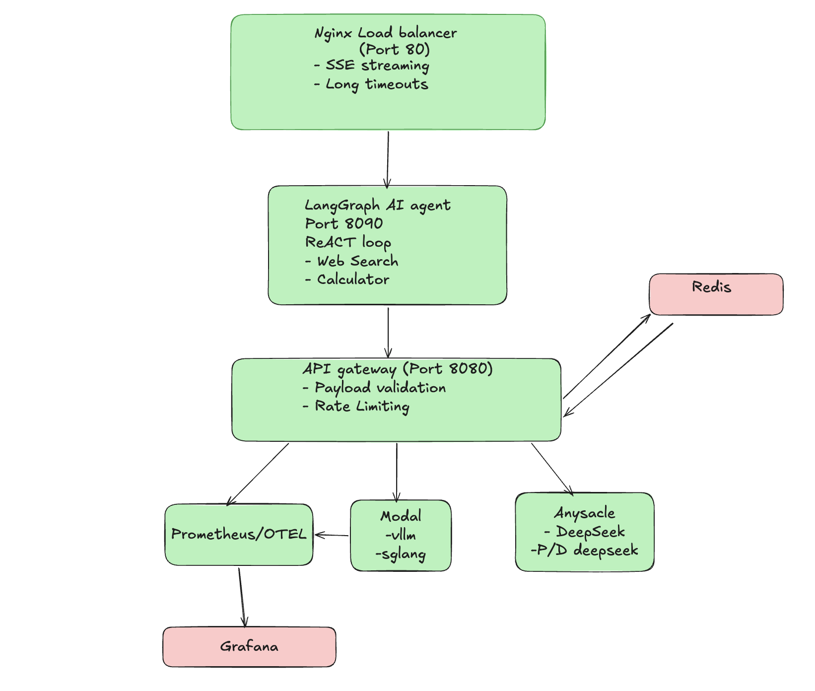{#fig-architecture fig-alt="Architecture diagram showing the full stack LLM inference pipeline with Nginx, LangGraph Agent, API Gateway, and various inference backends"}
**Layer Responsibilities:**
| Layer | Technology | Purpose |
|-------|------------|---------|
| Load Balancer | Nginx | SSE streaming, long timeouts for cold starts |
| Agent Layer | LangGraph | ReAct loop with tool calling (web search, calculator) |
| API Gateway | FastAPI | Request routing, backend selection, metrics |
| Inference | vLLM + Ray Serve | High-throughput model serving |
| Inference | Anyscale + P/D Moe | For Deepseek MOE model and disaggregated Prefill |
| Monitoring | Prometheus + Grafana | Real-time metrics and alerting |
### Why This Architecture?
1. **Nginx handles SSE complexity** - Streaming responses require careful timeout configuration
2. **Gateway enables multiple routes** - Route traffic between backends without client changes (Clients can choose their own config)
3. **Monitoring is essential** - You can't optimize what you don't measure
## Experiment Methodology
### Testing Phases
Our load testing follows a rigorous 4-phase methodology:
```{python}
#| label: methodology-diagram
#| fig-cap: "Load Testing Phases"
phases = pd.DataFrame({
    'Phase': ['Phase 0', 'Phase 1', 'Phase 2', 'Phase 3'],
    'Name': ['Warmup', 'Baseline', 'Concurrency Sweep', 'Sustained RPS'],
    'Description': [
        '5 requests to warm containers (results discarded)',
        'Sequential requests, varying prompt lengths',
        'Parallel requests: 1, 2, 4, 8, 16 concurrent',
        'Fixed rate: 1.0, 2.0, 5.0, 10.0 req/s for 30s each'
    ],
    'Purpose': [
        'Eliminate cold-start noise',
        'Establish single-request performance',
        'Find concurrency limits',
        'Test sustained production load'
    ]
})

fig = go.Figure(data=[go.Table(
    header=dict(
        values=['<b>Phase</b>', '<b>Name</b>', '<b>Description</b>', '<b>Purpose</b>'],
        fill_color='#2C3E50',
        font=dict(color='white', size=12),
        align='left'
    ),
    cells=dict(
        values=[phases[col] for col in phases.columns],
        fill_color='#F8F9FA',
        align='left',
        height=30
    )
)])
fig.update_layout(margin=dict(l=0, r=0, t=0, b=0), height=200)
fig.show()
```
### Metrics Collected
| Metric | Description | Why It Matters |
|--------|-------------|----------------|
| **TTFT** | Time to First Token | User-perceived responsiveness |
| **Total Latency** | End-to-end request time | SLA compliance |
| **Throughput** | Tokens per second | Cost efficiency |
| **TPOT** | Time per Output Token | Generation smoothness |
| **Success Rate** | % of completed requests | Reliability |
### Dataset
All experiments use the **ShareGPT** dataset:
- 500 conversations
- Input lengths: 100-2048 tokens
- Realistic multi-turn dialogue patterns
## Experiment 1: Qwen2.5-7B on Anyscale {#sec-qwen}
### Setup
- **Model:** Qwen2.5-7B-Instruct
- **Framework:** Ray Serve + vLLM
- **Infrastructure:** Anyscale managed cluster
- **GPU:** A10G
### Results
```{python}
#| label: qwen-concurrency
#| fig-cap: "Qwen2.5-7B Performance vs Concurrency"
# Filter out warmup row if present
qwen_data = qwen_results[qwen_results['concurrency'] > 0].copy()

fig = make_subplots(
    rows=2, cols=2,
    subplot_titles=(
        'TTFT by Concurrency',
        'Throughput by Concurrency',
        'Total Latency by Concurrency',
        'Success Rate'
    ),
    vertical_spacing=0.15
)

# TTFT
fig.add_trace(
    go.Scatter(x=qwen_data['concurrency'], y=qwen_data['ttft_p50_ms'],
               mode='lines+markers', name='TTFT p50', line=dict(color='#3498DB')),
    row=1, col=1
)
fig.add_trace(
    go.Scatter(x=qwen_data['concurrency'], y=qwen_data['ttft_p90_ms'],
               mode='lines+markers', name='TTFT p90', line=dict(color='#E74C3C', dash='dash')),
    row=1, col=1
)

# Throughput
fig.add_trace(
    go.Bar(x=qwen_data['concurrency'], y=qwen_data['throughput_tokens_per_sec'],
           name='Throughput', marker_color='#27AE60'),
    row=1, col=2
)

# Total Latency
fig.add_trace(
    go.Scatter(x=qwen_data['concurrency'], y=qwen_data['total_latency_p50_ms'],
               mode='lines+markers', name='Latency p50', line=dict(color='#9B59B6')),
    row=2, col=1
)
fig.add_trace(
    go.Scatter(x=qwen_data['concurrency'], y=qwen_data['total_latency_p90_ms'],
               mode='lines+markers', name='Latency p90', line=dict(color='#E67E22', dash='dash')),
    row=2, col=1
)

# Success Rate
success_rate = 100 - qwen_data['error_rate_%']
fig.add_trace(
    go.Bar(x=qwen_data['concurrency'], y=success_rate,
           name='Success %', marker_color='#1ABC9C'),
    row=2, col=2
)

fig.update_layout(height=600, showlegend=True, title_text="Qwen2.5-7B Performance Metrics")
fig.update_xaxes(title_text="Concurrency", row=2, col=1)
fig.update_xaxes(title_text="Concurrency", row=2, col=2)
fig.update_yaxes(title_text="ms", row=1, col=1)
fig.update_yaxes(title_text="tokens/sec", row=1, col=2)
fig.update_yaxes(title_text="ms", row=2, col=1)
fig.update_yaxes(title_text="%", row=2, col=2)
fig.show()
```
### Key Findings
::: {.callout-note}
## Qwen2.5-7B Performance Summary
- **100% success rate** across all concurrency levels (1-16)
- **TTFT p50:** 408-564ms (remarkably stable under load)
- **Throughput:** 34-37 tokens/sec
- **Graceful degradation:** Latency increases linearly, no cliff
:::
**Why Qwen for Production?**
1. **Reliability:** Zero failures even at 16 concurrent requests
2. **Tool Calling:** Excellent function-calling capabilities for agents
3. **Predictable Latency:** Easy to set SLAs with stable p90 metrics
## Experiment 2: DeepSeek MoE with Disaggregated Prefill {#sec-deepseek-disagg}
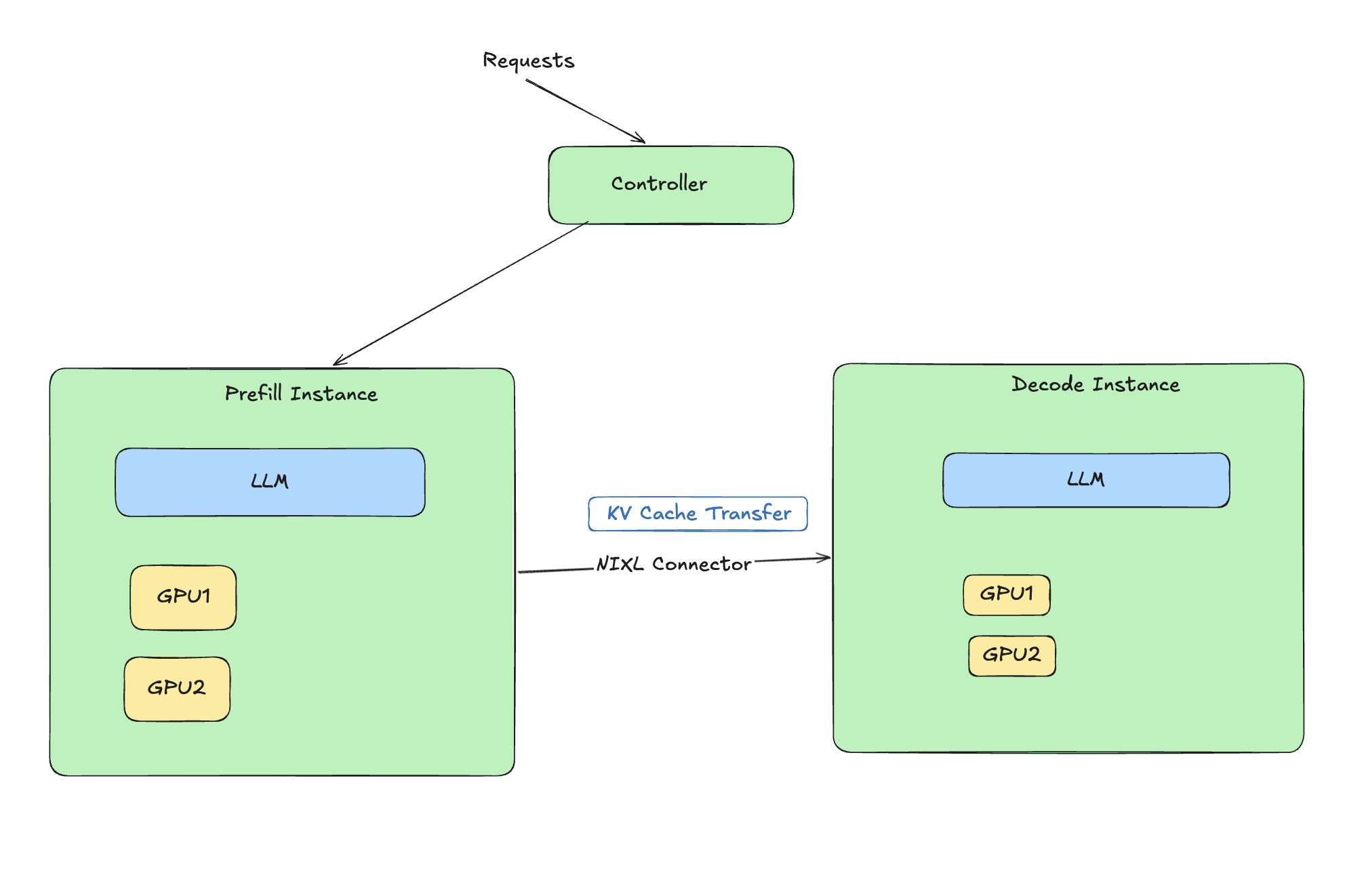{#fig-architecture fig-alt="Architecture diagram showing how disaggregated prefill decode works with NIXL connector"}
### What is Disaggregated Prefill?
LLM inference has two distinct phases:
1. **Prefill:** Process input tokens (compute-bound)
2. **Decode:** Generate output tokens one at a time (memory-bound)
**Disaggregated prefill** separates these phases onto different workers, allowing each to be optimized independently. This is especially beneficial for Mixture-of-Experts (MoE) models where expert routing adds complexity.
```{mermaid}
%%| fig-cap: "Disaggregated Prefill Architecture"
flowchart LR
Input[Input Tokens] --> Prefill[Prefill Workers<br/>Compute Optimized]
Prefill --> KV[KV Cache Transfer]
KV --> Decode[Decode Workers<br/>Memory Optimized]
Decode --> Output[Output Tokens]
```
### Setup
- **Model:** DeepSeek-V2-Lite-Chat (16B total, 2.4B active parameters)
- **Framework:** Ray Serve + vLLM with PD disaggregation
- **Infrastructure:** Anyscale (g5.12xlarge, 4x A10G)
### Results
```{python}
#| label: deepseek-disagg-results
#| fig-cap: "DeepSeek MoE with Disaggregated Prefill"
# Filter valid data
ds_data = deepseek_disagg[deepseek_disagg['concurrency'] > 0].copy()

fig = make_subplots(
    rows=1, cols=2,
    subplot_titles=('Throughput Comparison', 'TTFT Comparison')
)

fig.add_trace(
    go.Bar(x=ds_data['concurrency'], y=ds_data['throughput_tokens_per_sec'],
           name='DeepSeek (Disagg)', marker_color='#E74C3C'),
    row=1, col=1
)

fig.add_trace(
    go.Scatter(x=ds_data['concurrency'], y=ds_data['ttft_p50_ms'],
               mode='lines+markers', name='TTFT p50', line=dict(color='#3498DB')),
    row=1, col=2
)

fig.update_layout(height=400, title_text="DeepSeek-V2-Lite with Disaggregated Prefill")
fig.update_xaxes(title_text="Concurrency")
fig.update_yaxes(title_text="tokens/sec", row=1, col=1)
fig.update_yaxes(title_text="ms", row=1, col=2)
fig.show()
```
### Key Findings
::: {.callout-important}
## DeepSeek Disaggregated Performance
- **85 tokens/sec** at concurrency=1 (2.3x faster than Qwen!)
- **100% success rate** at all load levels
- **TTFT p50:** 406ms (comparable to Qwen)
- MoE efficiency unlocked through proper infrastructure
:::
## Experiment 3: DeepSeek WITHOUT Disaggregation {#sec-deepseek-no-disagg}
To demonstrate the impact of infrastructure choices, we ran the same DeepSeek model **without** disaggregated prefill.
### Results
<!-- TODO: Add CSV path when results are available -->
```{python}
#| label: deepseek-comparison
#| fig-cap: "Impact of Disaggregated Prefill on DeepSeek MoE"
#| eval: false
# This will be populated with actual non-disaggregated results
# For now, using documented values from moe-ray-deepseek-loadtest-result.md

comparison_data = pd.DataFrame({
    'Configuration': ['With Disaggregation', 'Without Disaggregation'],
    'Throughput (tok/s)': [85.1, 6.6],
    'TTFT p50 (ms)': [406, 5028],
    'Success Rate (%)': [100, 64.7],
    'Max Stable RPS': [10.0, 2.0]
})

fig = make_subplots(
    rows=2, cols=2,
    subplot_titles=('Throughput', 'TTFT', 'Success Rate', 'Max Stable RPS'),
    specs=[[{"type": "bar"}, {"type": "bar"}],
           [{"type": "bar"}, {"type": "bar"}]]
)

colors = ['#27AE60', '#E74C3C']

fig.add_trace(go.Bar(x=comparison_data['Configuration'],
                     y=comparison_data['Throughput (tok/s)'],
                     marker_color=colors), row=1, col=1)
fig.add_trace(go.Bar(x=comparison_data['Configuration'],
                     y=comparison_data['TTFT p50 (ms)'],
                     marker_color=colors), row=1, col=2)
fig.add_trace(go.Bar(x=comparison_data['Configuration'],
                     y=comparison_data['Success Rate (%)'],
                     marker_color=colors), row=2, col=1)
fig.add_trace(go.Bar(x=comparison_data['Configuration'],
                     y=comparison_data['Max Stable RPS'],
                     marker_color=colors), row=2, col=2)

fig.update_layout(height=500, showlegend=False,
                  title_text="Disaggregated vs Non-Disaggregated Prefill")
fig.show()
```
### The Shocking Difference
| Metric | With Disaggregation | Without | Difference |
|--------|---------------------|---------|------------|
| Throughput | 85.1 tok/s | 6.6 tok/s | **13x slower** |
| TTFT p50 | 406ms | 5,028ms | **12x slower** |
| Success Rate | 100% | 64.7% | **35% more failures** |
| Max Stable RPS | 10.0 | 2.0 | **5x lower** |
::: {.callout-warning}
## Critical Infrastructure Insight
The **same model** showed 13x throughput difference based solely on whether disaggregated prefill was enabled. This demonstrates that infrastructure choices can matter more than model selection.
:::
## Experiment 4: LLaMA 3.1-8B with LMCache on Modal {#sec-modal}
### Setup
- **Model:** LLaMA 3.1-8B with LMCache (prefix caching)
- **Framework:** vLLM on Modal (serverless)
- **Optimization:** Prefix caching for repeated prompts
### Results
```{python}
#| label: modal-results
#| fig-cap: "LLaMA 3.1-8B with LMCache on Modal"
modal_data = modal_lmcache[modal_lmcache['concurrency'] > 0].copy()

fig = make_subplots(rows=1, cols=2,
                    subplot_titles=('Throughput', 'TTFT'))

fig.add_trace(
    go.Bar(x=modal_data['concurrency'], y=modal_data['throughput_tokens_per_sec'],
           marker_color='#9B59B6'),
    row=1, col=1
)

fig.add_trace(
    go.Scatter(x=modal_data['concurrency'], y=modal_data['ttft_p50_ms'],
               mode='lines+markers', line=dict(color='#E67E22')),
    row=1, col=2
)

fig.update_layout(height=350, title_text="Modal + LMCache Performance")
fig.update_xaxes(title_text="Concurrency")
fig.show()
```
### Key Findings
- **Max sustainable:** ~4 concurrent requests
- **Throughput:** 25-26 tokens/sec
- **Fails at:** >1.0 RPS sustained load
### Trade-offs
| Pros | Cons |
|------|------|
| Scale-to-zero (cost savings) | Cold start latency |
| Simple deployment | Lower throughput ceiling |
| Good for bursty workloads | Not suitable for sustained load |
## Head-to-Head Comparison {#sec-comparison}
```{python}
#| label: final-comparison
#| fig-cap: "Complete Model Comparison"
comparison = pd.DataFrame({
    'Model': ['Qwen2.5-7B', 'DeepSeek (Disagg)', 'DeepSeek (No Disagg)', 'LLaMA+LMCache'],
    'Throughput': [37, 85, 6.6, 26],
    'TTFT_p50': [408, 406, 5028, 1048],
    'Max_RPS': [10.0, 10.0, 2.0, 1.0],
    'Success_Rate': [100, 100, 64.7, 75]
})

fig = make_subplots(
    rows=2, cols=2,
    subplot_titles=('Peak Throughput (tok/s)', 'TTFT p50 (ms)',
                    'Max Stable RPS', 'Success Rate (%)'),
    vertical_spacing=0.15
)

colors = ['#3498DB', '#E74C3C', '#95A5A6', '#9B59B6']

fig.add_trace(go.Bar(x=comparison['Model'], y=comparison['Throughput'],
                     marker_color=colors), row=1, col=1)
fig.add_trace(go.Bar(x=comparison['Model'], y=comparison['TTFT_p50'],
                     marker_color=colors), row=1, col=2)
fig.add_trace(go.Bar(x=comparison['Model'], y=comparison['Max_RPS'],
                     marker_color=colors), row=2, col=1)
fig.add_trace(go.Bar(x=comparison['Model'], y=comparison['Success_Rate'],
                     marker_color=colors), row=2, col=2)

fig.update_layout(height=600, showlegend=False,
                  title_text="Model Performance Comparison")
fig.update_xaxes(tickangle=45)
fig.show()
```
### Summary Table
| Metric | Qwen2.5-7B | DeepSeek (Disagg) | DeepSeek (No Disagg) | LLaMA+LMCache |
|--------|------------|-------------------|----------------------|---------------|
| **Peak Throughput** | 37 tok/s | **85 tok/s** | 6.6 tok/s | 26 tok/s |
| **TTFT p50** | 408ms | **406ms** | 5,028ms | 1,048ms |
| **Max Stable RPS** | **10.0** | **10.0** | 2.0 | <1.0 |
| **Success Rate** | **100%** | **100%** | 64.7% | ~75% |
| **Best For** | Production APIs | High throughput | Avoid | Cost savings |
## Recommendations {#sec-recommendations}
### Decision Matrix
```{mermaid}
%%| fig-cap: "Choosing Your Inference Stack"
flowchart TD
Start[What's your priority?] --> Cost{Cost Sensitive?}
Cost -->|Yes| Bursty{Bursty Traffic?}
Bursty -->|Yes| Modal[Modal + LMCache]
Bursty -->|No| Qwen[Qwen on Anyscale]
Cost -->|No| Throughput{Need Max Throughput?}
Throughput -->|Yes| DeepSeek[DeepSeek + Disagg Prefill]
Throughput -->|No| Tools{Need Tool Calling?}
Tools -->|Yes| Qwen
Tools -->|No| DeepSeek
```
### When to Use What
1. **Production APIs with tool-calling:** Qwen2.5-7B on Ray Serve
- Highest reliability (100% success)
- Excellent function-calling support
- Predictable latency for SLAs
2. **Maximum throughput batch processing:** DeepSeek with disaggregated prefill
- 2.3x faster than alternatives
- Cost-efficient for high-volume workloads
3. **Cost-sensitive, bursty workloads:** Modal + LMCache
- Scale-to-zero saves money during idle periods
- Good for development and testing
4. **Avoid:** Non-disaggregated MoE deployments
- 13x throughput penalty is rarely acceptable
## Lessons Learned {#sec-lessons}
::: {.callout-note}
## Key Takeaways
1. **Infrastructure choices matter as much as model selection** - The same model showed 13x performance difference based on deployment strategy
2. **MoE models need disaggregated prefill** - Without it, you're leaving 90%+ of performance on the table
3. **Test under realistic load patterns** - Single-request benchmarks don't reveal concurrency limits
4. **Monitor TTFT separately from total latency** - Users perceive TTFT as responsiveness
5. **Serverless has trade-offs** - Great for cost, but cold starts and throughput ceilings matter
:::
## Future Experiments {#sec-future}
<!-- TODO: Add results as experiments are completed -->
### Planned Experiments
- [ ] **Cost Analysis:** $/1M tokens comparison across platforms
- [ ] **Speculative Decoding:** Draft model acceleration
- [ ] **Quantization Impact:** AWQ/GPTQ throughput vs quality
- [ ] **Long Context:** 8K, 16K, 32K token performance
- [ ] **Agent Latency:** End-to-end tool-calling benchmarks
- [ ] **SGLang vs vLLM:** Direct framework comparison
- [ ] **Chunked Prefill:** Alternative to disaggregation
## Appendix: Reproduction {#sec-appendix}
### Repository
All code, deployment scripts, and results are available at:
<https://github.com/vinayhpandya/simple_full_stack_inference>
### Running Load Tests
```bash
# Install dependencies
uv sync

# Run load test against your endpoint
python load_test.py \
    --endpoint "https://your-endpoint.com/v1/chat/completions" \
    --model "qwen2.5-7b-instruct" \
    --dataset sharegpt \
    --concurrency-levels 1 2 4 8 16
```
### Deployment Commands
::: {.panel-tabset}
## Modal
```bash
modal deploy modal_vllm_deploy.py
```
## Anyscale
```bash
anyscale service deploy anyscale_deepseek_deploy.py
```
## Local Gateway
```bash
python gateway_launcher.py --config gateway_config.yaml
```
:::
---
*Generated with benchmarking infrastructure from the simple_full_stack_inference project.*

