---
title: "Building a Production-Grade LLM Inference Stack: Benchmarking vLLM, Ray Serve, and MoE Models"
author:
- "Vinay Pandya"
- "Yiran Xu"
date: "2026-04-25"
categories: [llm, inference, vllm, ray-serve, moe, benchmarking, deep-learning]
toc: true
toc-depth: 3
number-sections: true
highlight-style: github
code-fold: true
code-tools: true
execute:
eval: true
warning: false
message: false
---
```{python}
#| label: setup
#| include: false
import pandas as pd
import plotly.express as px
import plotly.graph_objects as go
from plotly.subplots import make_subplots
import numpy as np
# Set default plotly template
import plotly.io as pio
pio.templates.default = "plotly_white"
# Load all result CSVs
qwen_results = pd.read_csv("../results/qwen_vllm_model_sharegpt_concurrency_20260411_131143.csv")
deepseek_disagg = pd.read_csv("../results/deepseek_sharegpt_concurrency_20260411_132403.csv")
modal_lmcache = pd.read_csv("../results/modal_vllm_lmcache_sharegpt_concurrency_20260408_141225.csv")
# Note: Add path for non-disaggregated DeepSeek results when available
```
## Introduction
These are our notes from benchmarking a self-hosted LLM inference stack. The goal was practical: figure out which combination of model, serving framework, and infrastructure actually holds up under realistic load, and where the real trade-offs are.
I tested four configurations:
- **Qwen2.5-7B** on Ray Serve + vLLM (production baseline)
- **DeepSeek-V2-Lite MoE** with disaggregated prefill
- **DeepSeek-V2-Lite MoE** without disaggregated prefill
- **LLaMA 3.1-8B** with LMCache on Modal (serverless)
The finding that surprised me most: the same DeepSeek model showed a 13x throughput difference depending solely on whether disaggregated prefill was enabled. That's not a model choice — it's a configuration choice, and it's easy to get wrong.
## Architecture Overview
### The Full Stack
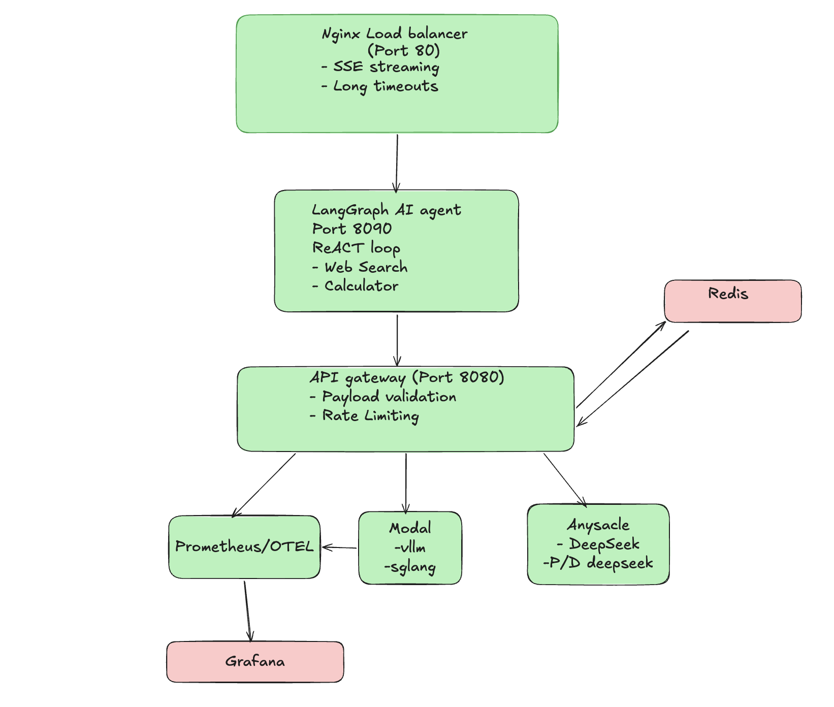{#fig-architecture fig-alt="Architecture diagram showing the full stack LLM inference pipeline with Nginx, LangGraph Agent, API Gateway, and various inference backends"}
**Layer Responsibilities:**
| Layer | Technology | Purpose |
|-------|------------|---------|
| Load Balancer | Nginx | SSE streaming, long timeouts for cold starts |
| Agent Layer | LangGraph | ReAct loop with tool calling (web search, calculator) |
| API Gateway | FastAPI | Request routing, backend selection, metrics |
| Inference | vLLM + Ray Serve | High-throughput model serving |
| Monitoring | Prometheus + Grafana | Real-time metrics and alerting |
### Why This Architecture?
A few decisions worth noting. Nginx sits at the front because SSE streaming requires careful timeout handling that most default configs don't cover. The FastAPI gateway makes it straightforward to swap inference backends without changing anything on the client side. And running Prometheus from the start, even during experiments, meant I could catch degradation as it happened rather than reconstructing it from logs.
## Experiment Methodology
### Testing Phases
```{python}
#| label: methodology-diagram
#| fig-cap: "Load Testing Phases"
phases = pd.DataFrame({
    'Phase': ['Phase 0', 'Phase 1', 'Phase 2', 'Phase 3'],
    'Name': ['Warmup', 'Baseline', 'Concurrency Sweep', 'Sustained RPS'],
    'Description': [
        '5 requests to warm containers (results discarded)',
        'Sequential requests, varying prompt lengths',
        'Parallel requests: 1, 2, 4, 8, 16 concurrent',
        'Fixed rate: 1.0, 2.0, 5.0, 10.0 req/s for 30s each'
    ],
    'Purpose': [
        'Eliminate cold-start noise',
        'Establish single-request performance',
        'Find concurrency limits',
        'Test sustained production load'
    ]
})

fig = go.Figure(data=[go.Table(
    header=dict(
        values=['<b>Phase</b>', '<b>Name</b>', '<b>Description</b>', '<b>Purpose</b>'],
        fill_color='#2C3E50',
        font=dict(color='white', size=12),
        align='left',
        height=35
    ),
    cells=dict(
        values=[phases[col] for col in phases.columns],
        fill_color=[['#F8F9FA', '#FFFFFF'] * 2],
        align='left',
        height=32,
        font=dict(size=11)
    )
)])
fig.update_layout(margin=dict(l=0, r=0, t=10, b=10), height=180)
fig.show()
```
### Metrics Collected
| Metric | Description | Why It Matters |
|--------|-------------|----------------|
| **TTFT** | Time to First Token | User-perceived responsiveness |
| **Total Latency** | End-to-end request time | SLA compliance |
| **Throughput** | Tokens per second | Cost efficiency |
| **TPOT** | Time per Output Token | Generation smoothness |
| **Success Rate** | % of completed requests | Reliability |
### Dataset
All experiments use the **ShareGPT** dataset:
- 500 conversations
- Input lengths: 100-2048 tokens
- Realistic multi-turn dialogue patterns
## Experiment 1: Qwen2.5-7B on Anyscale {#sec-qwen}
### Setup
- **Model:** Qwen2.5-7B-Instruct
- **Framework:** Ray Serve + vLLM
- **Infrastructure:** Anyscale managed cluster
- **GPU:** A10G
### Results
```{python}
#| label: qwen-concurrency
#| fig-cap: "Qwen2.5-7B Performance vs Concurrency"
# Filter out warmup row if present
qwen_data = qwen_results[qwen_results['concurrency'] > 0].copy()

fig = make_subplots(
    rows=2, cols=2,
    subplot_titles=(
        '<b>TTFT (Time to First Token)</b>',
        '<b>Throughput</b>',
        '<b>End-to-End Latency</b>',
        '<b>Success Rate</b>'
    ),
    vertical_spacing=0.18,
    horizontal_spacing=0.12
)

# TTFT
fig.add_trace(
    go.Scatter(x=qwen_data['concurrency'], y=qwen_data['ttft_p50_ms'],
               mode='lines+markers', name='p50', line=dict(color='#3498DB', width=2),
               marker=dict(size=8), legendgroup='ttft', legendgrouptitle_text='TTFT'),
    row=1, col=1
)
fig.add_trace(
    go.Scatter(x=qwen_data['concurrency'], y=qwen_data['ttft_p90_ms'],
               mode='lines+markers', name='p90', line=dict(color='#E74C3C', width=2, dash='dash'),
               marker=dict(size=8), legendgroup='ttft'),
    row=1, col=1
)

# Throughput
fig.add_trace(
    go.Bar(x=qwen_data['concurrency'], y=qwen_data['throughput_tokens_per_sec'],
           name='Tokens/sec', marker_color='#27AE60', showlegend=False),
    row=1, col=2
)

# Total Latency
fig.add_trace(
    go.Scatter(x=qwen_data['concurrency'], y=qwen_data['latency_p50_ms'],
               mode='lines+markers', name='p50', line=dict(color='#9B59B6', width=2),
               marker=dict(size=8), legendgroup='latency', legendgrouptitle_text='Latency'),
    row=2, col=1
)
fig.add_trace(
    go.Scatter(x=qwen_data['concurrency'], y=qwen_data['latency_p90_ms'],
               mode='lines+markers', name='p90', line=dict(color='#E67E22', width=2, dash='dash'),
               marker=dict(size=8), legendgroup='latency'),
    row=2, col=1
)

# Success Rate
success_rate = 100 - qwen_data['error_rate_%']
fig.add_trace(
    go.Bar(x=qwen_data['concurrency'], y=success_rate,
           name='Success %', marker_color='#1ABC9C', showlegend=False),
    row=2, col=2
)

fig.update_layout(
    height=550,
    showlegend=True,
    legend=dict(orientation='h', yanchor='bottom', y=1.02, xanchor='center', x=0.5),
    margin=dict(t=80, b=60, l=60, r=40),
    font=dict(size=11)
)

# Update all axes
fig.update_xaxes(title_text="Concurrency", row=1, col=1, tickmode='array', tickvals=qwen_data['concurrency'])
fig.update_xaxes(title_text="Concurrency", row=1, col=2, tickmode='array', tickvals=qwen_data['concurrency'])
fig.update_xaxes(title_text="Concurrency", row=2, col=1, tickmode='array', tickvals=qwen_data['concurrency'])
fig.update_xaxes(title_text="Concurrency", row=2, col=2, tickmode='array', tickvals=qwen_data['concurrency'])
fig.update_yaxes(title_text="Milliseconds", row=1, col=1)
fig.update_yaxes(title_text="Tokens/sec", row=1, col=2)
fig.update_yaxes(title_text="Milliseconds", row=2, col=1)
fig.update_yaxes(title_text="Percent", row=2, col=2, range=[0, 105])

fig.show()
```
### Key Findings
::: {.callout-note}
## Qwen2.5-7B Performance Summary
- **100% success rate** across all concurrency levels (1–16)
- **TTFT p50:** 408–564ms, stable across load levels
- **Throughput:** 34–37 tokens/sec, essentially flat
- Latency increases linearly with concurrency — no sudden cliff
:::
Qwen held up well. What I didn't expect was how flat the throughput curve stayed — it didn't gain much as concurrency increased, but it also didn't degrade. The linear latency scaling makes it straightforward to set SLAs: if p50 is 408ms at concurrency 1, you can roughly estimate what it'll look like at higher load without surprises.
Its tool-calling reliability is also notably good, which matters for the agent layer. This is why it's the production baseline.
## Experiment 2: DeepSeek MoE with Disaggregated Prefill {#sec-deepseek-disagg}
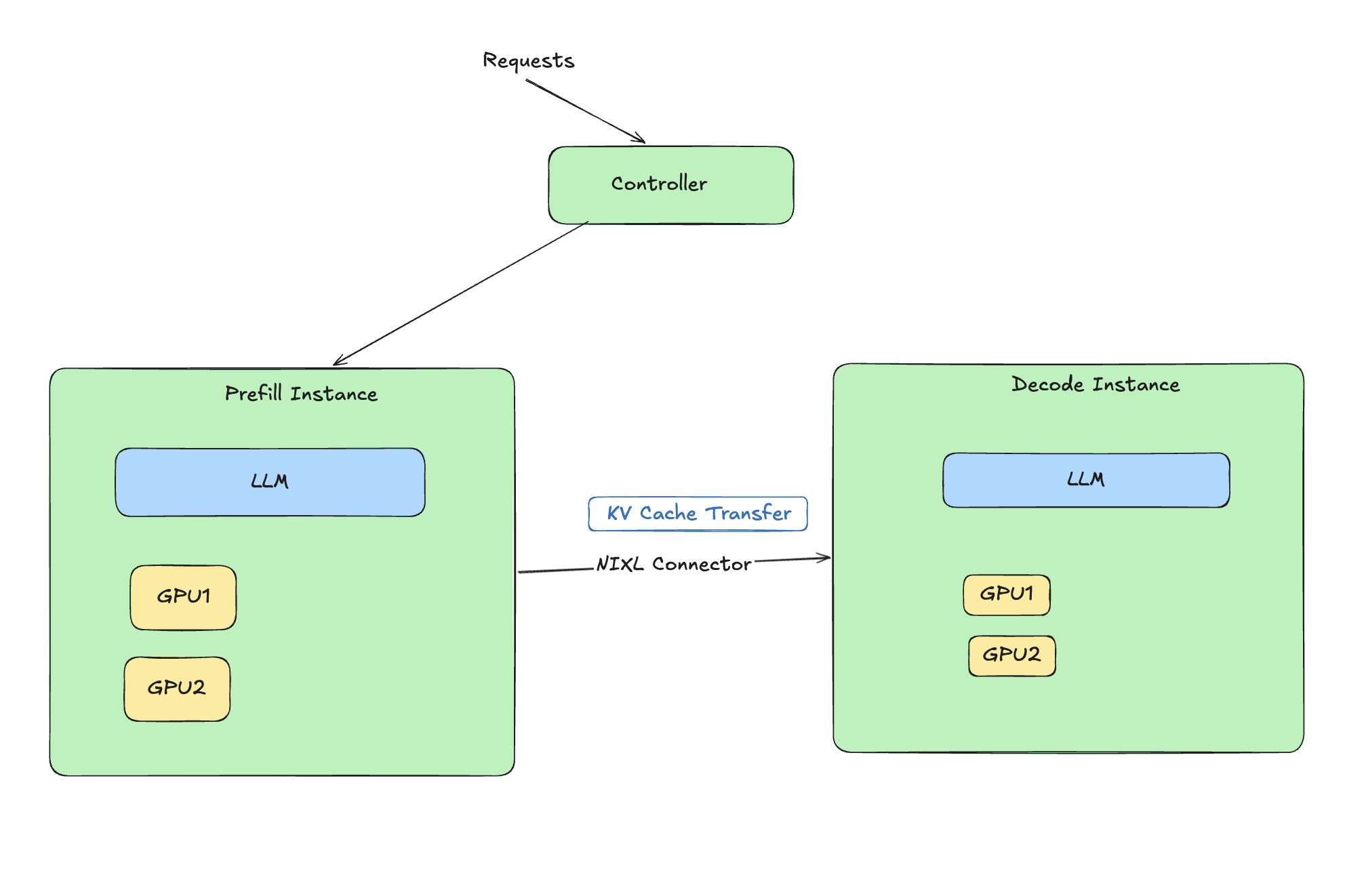{#fig-architecture fig-alt="Architecture diagram showing how disaggregated prefill decode works with NIXL connector"}
### What is Disaggregated Prefill?
LLM inference has two distinct phases:
1. **Prefill:** Process input tokens (compute-bound)
2. **Decode:** Generate output tokens one at a time (memory-bound)
These phases have very different resource profiles. Disaggregated prefill separates them onto different workers so each can be tuned independently. For MoE models, this matters more than usual — expert routing during prefill adds overhead that gets in the way of efficient decoding if both phases share the same worker.
```{mermaid}
%%| eval: true
%%| fig-cap: "Disaggregated Prefill Architecture"
flowchart LR
    Input[Input Tokens] --> Prefill[Prefill Workers<br/>Compute Optimized]
    Prefill --> KV[KV Cache Transfer]
    KV --> Decode[Decode Workers<br/>Memory Optimized]
    Decode --> Output[Output Tokens]
```
### Setup
- **Model:** DeepSeek-V2-Lite-Chat (16B total, 2.4B active parameters)
- **Framework:** Ray Serve + vLLM with PD disaggregation
- **Infrastructure:** Anyscale (g5.12xlarge, 4x A10G)
### Results
```{python}
#| label: deepseek-disagg-results
#| fig-cap: "DeepSeek MoE with Disaggregated Prefill"
# Filter valid data
ds_data = deepseek_disagg[deepseek_disagg['concurrency'] > 0].copy()

fig = make_subplots(
    rows=1, cols=2,
    subplot_titles=('<b>Throughput</b>', '<b>Time to First Token</b>'),
    horizontal_spacing=0.15
)

fig.add_trace(
    go.Bar(x=ds_data['concurrency'], y=ds_data['throughput_tokens_per_sec'],
           name='Throughput', marker_color='#E74C3C', showlegend=False),
    row=1, col=1
)

fig.add_trace(
    go.Scatter(x=ds_data['concurrency'], y=ds_data['ttft_p50_ms'],
               mode='lines+markers', name='TTFT p50',
               line=dict(color='#3498DB', width=2), marker=dict(size=8), showlegend=False),
    row=1, col=2
)

fig.update_layout(
    height=350,
    margin=dict(t=60, b=60, l=60, r=40),
    font=dict(size=11)
)
fig.update_xaxes(title_text="Concurrency", tickmode='array', tickvals=ds_data['concurrency'])
fig.update_yaxes(title_text="Tokens/sec", row=1, col=1)
fig.update_yaxes(title_text="Milliseconds", row=1, col=2)
fig.show()
```
### Key Findings
::: {.callout-important}
## DeepSeek Disaggregated Performance
- **85 tokens/sec** at concurrency=1 — 2.3x higher than Qwen
- **100% success rate** across all load levels
- **TTFT p50:** 406ms, on par with Qwen despite a much larger model
- MoE efficiency only materializes with the right infrastructure
:::
The throughput number was the clearest result from the whole experiment. 85 tokens/sec from a 16B-parameter model, with TTFT matching a 7B model, is only possible because the disaggregated setup lets the prefill and decode workers each do what they're actually good at. Without it, the picture is very different — see the next section.
## Experiment 3: DeepSeek WITHOUT Disaggregation {#sec-deepseek-no-disagg}
I ran the same DeepSeek model without disaggregated prefill to make the comparison concrete.
### Results
<!-- TODO: Add CSV path when results are available -->
```{python}
#| label: deepseek-comparison
#| fig-cap: "Impact of Disaggregated Prefill on DeepSeek MoE"
#| eval: false
# This will be populated with actual non-disaggregated results
# For now, using documented values from moe-ray-deepseek-loadtest-result.md

comparison_data = pd.DataFrame({
    'Configuration': ['With Disaggregation', 'Without Disaggregation'],
    'Throughput (tok/s)': [85.1, 6.6],
    'TTFT p50 (ms)': [406, 5028],
    'Success Rate (%)': [100, 64.7],
    'Max Stable RPS': [10.0, 2.0]
})

fig = make_subplots(
    rows=2, cols=2,
    subplot_titles=('Throughput', 'TTFT', 'Success Rate', 'Max Stable RPS'),
    specs=[[{"type": "bar"}, {"type": "bar"}],
           [{"type": "bar"}, {"type": "bar"}]]
)

colors = ['#27AE60', '#E74C3C']

fig.add_trace(go.Bar(x=comparison_data['Configuration'],
                     y=comparison_data['Throughput (tok/s)'],
                     marker_color=colors), row=1, col=1)
fig.add_trace(go.Bar(x=comparison_data['Configuration'],
                     y=comparison_data['TTFT p50 (ms)'],
                     marker_color=colors), row=1, col=2)
fig.add_trace(go.Bar(x=comparison_data['Configuration'],
                     y=comparison_data['Success Rate (%)'],
                     marker_color=colors), row=2, col=1)
fig.add_trace(go.Bar(x=comparison_data['Configuration'],
                     y=comparison_data['Max Stable RPS'],
                     marker_color=colors), row=2, col=2)

fig.update_layout(height=500, showlegend=False,
                  title_text="Disaggregated vs Non-Disaggregated Prefill")
fig.show()
```
### The Difference
| Metric | With Disaggregation | Without | Difference |
|--------|---------------------|---------|------------|
| Throughput | 85.1 tok/s | 6.6 tok/s | **13x slower** |
| TTFT p50 | 406ms | 5,028ms | **12x slower** |
| Success Rate | 100% | 64.7% | **35% more failures** |
| Max Stable RPS | 10.0 | 2.0 | **5x lower** |
::: {.callout-warning}
## Infrastructure vs Model Choice
This is the same model, same hardware, different configuration. The 13x throughput gap isn't about the model — it's about whether the serving infrastructure matches how MoE models actually work. Picking a MoE model without accounting for this will result in significantly worse performance than a smaller dense model.
:::
## Experiment 4: LLaMA 3.1-8B with LMCache on Modal {#sec-modal}
### Setup
- **Model:** LLaMA 3.1-8B with LMCache (prefix caching)
- **Framework:** vLLM on Modal (serverless)
- **Optimization:** Prefix caching for repeated prompts
### Results
```{python}
#| label: modal-results
#| fig-cap: "LLaMA 3.1-8B with LMCache on Modal"
modal_data = modal_lmcache[modal_lmcache['concurrency'] > 0].copy()

fig = make_subplots(
    rows=1, cols=2,
    subplot_titles=('<b>Throughput</b>', '<b>Time to First Token</b>'),
    horizontal_spacing=0.15
)

fig.add_trace(
    go.Bar(x=modal_data['concurrency'], y=modal_data['throughput_tokens_per_sec'],
           marker_color='#9B59B6', showlegend=False),
    row=1, col=1
)

fig.add_trace(
    go.Scatter(x=modal_data['concurrency'], y=modal_data['ttft_p50_ms'],
               mode='lines+markers', line=dict(color='#E67E22', width=2),
               marker=dict(size=8), showlegend=False),
    row=1, col=2
)

fig.update_layout(
    height=350,
    margin=dict(t=60, b=60, l=60, r=40),
    font=dict(size=11)
)
fig.update_xaxes(title_text="Concurrency", tickmode='array', tickvals=modal_data['concurrency'])
fig.update_yaxes(title_text="Tokens/sec", row=1, col=1)
fig.update_yaxes(title_text="Milliseconds", row=1, col=2)
fig.show()
```
### Key Findings
Modal's serverless deployment caps out around 4 concurrent requests, with throughput between 25–26 tokens/sec. It starts failing above 1.0 RPS on sustained load. The cold start penalty is real, and it shows up in the TTFT numbers under anything resembling steady traffic.
That said, scale-to-zero is a meaningful cost advantage if your workload is bursty. For development, testing, or low-traffic use cases where you're not running requests continuously, you won't pay for idle GPU time. That trade-off just doesn't work for anything that needs consistent throughput.
### Trade-offs
| Pros | Cons |
|------|------|
| Scale-to-zero (cost savings) | Cold start latency |
| Simple deployment | Lower throughput ceiling |
| Good for bursty workloads | Not suitable for sustained load |
## Head-to-Head Comparison {#sec-comparison}
```{python}
#| label: final-comparison
#| fig-cap: "Complete Model Comparison"
comparison = pd.DataFrame({
    'Model': ['Qwen2.5', 'DeepSeek-p/D', 'DeepSeek', 'LMCache'],
    'Throughput': [37, 85, 6.6, 26],
    'TTFT_p50': [408, 406, 5028, 1048],
    'Max_RPS': [10.0, 10.0, 2.0, 1.0],
    'Success_Rate': [100, 100, 64.7, 75]
})

fig = make_subplots(
    rows=2, cols=2,
    subplot_titles=(
        '<b>Peak Throughput</b>',
        '<b>TTFT p50</b>',
        '<b>Max Stable RPS</b>',
        '<b>Success Rate</b>'
    ),
    vertical_spacing=0.20,
    horizontal_spacing=0.12
)

colors = ['#3498DB', '#27AE60', '#E74C3C', '#9B59B6']

fig.add_trace(go.Bar(x=comparison['Model'], y=comparison['Throughput'],
                     marker_color=colors, showlegend=False,
                     text=comparison['Throughput'], textposition='outside'), row=1, col=1)
fig.add_trace(go.Bar(x=comparison['Model'], y=comparison['TTFT_p50'],
                     marker_color=colors, showlegend=False,
                     text=comparison['TTFT_p50'], textposition='outside'), row=1, col=2)
fig.add_trace(go.Bar(x=comparison['Model'], y=comparison['Max_RPS'],
                     marker_color=colors, showlegend=False,
                     text=comparison['Max_RPS'], textposition='outside'), row=2, col=1)
fig.add_trace(go.Bar(x=comparison['Model'], y=comparison['Success_Rate'],
                     marker_color=colors, showlegend=False,
                     text=comparison['Success_Rate'].apply(lambda x: f'{x}%'), textposition='outside'), row=2, col=2)

fig.update_layout(
    height=550,
    showlegend=False,
    margin=dict(t=60, b=80, l=60, r=40),
    font=dict(size=11)
)
fig.update_xaxes(tickangle=0)
fig.update_yaxes(title_text="Tokens/sec", row=1, col=1)
fig.update_yaxes(title_text="Milliseconds", row=1, col=2)
fig.update_yaxes(title_text="Requests/sec", row=2, col=1)
fig.update_yaxes(title_text="Percent", row=2, col=2, range=[0, 110])
fig.show()
```
### Summary Table
| Metric | Qwen2.5-7B | DeepSeek (Disagg) | DeepSeek (No Disagg) | LLaMA+LMCache |
|--------|------------|-------------------|----------------------|---------------|
| **Peak Throughput** | 37 tok/s | **85 tok/s** | 6.6 tok/s | 26 tok/s |
| **TTFT p50** | 408ms | **406ms** | 5,028ms | 1,048ms |
| **Max Stable RPS** | **10.0** | **10.0** | 2.0 | <1.0 |
| **Success Rate** | **100%** | **100%** | 64.7% | ~75% |
| **Best For** | Production APIs | High throughput | Avoid | Cost savings |
## Recommendations {#sec-recommendations}
### Decision Matrix
```{mermaid}
%%| eval: true
%%| fig-cap: "Choosing Your Inference Stack"
flowchart TD
    Start[What's your priority?] --> Cost{Cost Sensitive?}
    Cost -->|Yes| Bursty{Bursty Traffic?}
    Bursty -->|Yes| Modal[Modal + LMCache]
    Bursty -->|No| Qwen[Qwen on Anyscale]
    Cost -->|No| Throughput{Need Max Throughput?}
    Throughput -->|Yes| DeepSeek[DeepSeek + Disagg Prefill]
    Throughput -->|No| Tools{Need Tool Calling?}
    Tools -->|Yes| Qwen
    Tools -->|No| DeepSeek
```
### When to Use What
1. **Production APIs with tool-calling:** Qwen2.5-7B on Ray Serve
- Highest reliability (100% success)
- Excellent function-calling support
- Predictable latency for SLAs
2. **Maximum throughput batch processing:** DeepSeek with disaggregated prefill
- 2.3x faster than alternatives
- Cost-efficient for high-volume workloads
3. **Cost-sensitive, bursty workloads:** Modal + LMCache
- Scale-to-zero saves money during idle periods
- Good for development and testing
4. **Avoid:** Non-disaggregated MoE deployments
- 13x throughput penalty is rarely acceptable
## Lessons Learned {#sec-lessons}
::: {.callout-note}
## Key Takeaways
1. **Infrastructure configuration can outweigh model selection.** The DeepSeek results make this point clearly — a misconfigured 16B model underperformed a well-configured 7B model on every metric.
2. **MoE models require disaggregated prefill to reach their potential.** Without it, the prefill and decode phases compete for the same resources, and you end up with the worst of both.
3. **Single-request benchmarks are not enough.** The concurrency sweep and sustained RPS phases revealed limits that didn't show up at low load.
4. **TTFT and total latency tell different stories.** A model can have acceptable total latency but poor TTFT, which matters a lot for interactive use cases where users are waiting for the stream to start.
5. **Serverless is a cost tool, not a performance tool.** Modal is useful when GPU utilization would otherwise be near zero. It's not a substitute for a properly configured persistent cluster under real load.
:::
## Conclusions {#sec-conclusions}
If I had to distill this down: for a production API with tool-calling requirements, Qwen2.5-7B on Ray Serve is the most reliable option based on these experiments. If throughput is the priority and you're willing to configure it correctly, DeepSeek with disaggregated prefill is clearly the better choice. The serverless option on Modal works for specific cost scenarios but has real ceiling constraints that rule it out for sustained workloads.
The most important thing these experiments confirmed is that getting the infrastructure right matters as much as picking the right model. The difference between a well-configured and a poorly-configured MoE deployment is not marginal — it's the difference between a useful system and one that fails a third of its requests.
## Future Experiments {#sec-future}
### Planned
- [ ] **Cost Analysis:** $/1M tokens comparison across platforms
- [ ] **Speculative Decoding:** Draft model acceleration
- [ ] **Quantization Impact:** AWQ/GPTQ throughput vs quality
- [ ] **Long Context:** 8K, 16K, 32K token performance
- [ ] **Agent Latency:** End-to-end tool-calling benchmarks
- [ ] **SGLang vs vLLM:** Direct framework comparison
- [ ] **Chunked Prefill:** Alternative to disaggregation
## Appendix: Reproduction {#sec-appendix}
### Repository
All code, deployment scripts, and results are available at:
<https://github.com/vinayhpandya/simple_full_stack_inference>
### Running Load Tests
```bash
# Install dependencies
uv sync

# Run load test against your endpoint
python load_test.py \
    --endpoint "https://your-endpoint.com/v1/chat/completions" \
    --model "qwen2.5-7b-instruct" \
    --dataset sharegpt \
    --concurrency-levels 1 2 4 8 16
```
### Deployment Commands
::: {.panel-tabset}
## Modal
```bash
modal deploy modal_vllm_deploy.py
```
## Anyscale
```bash
anyscale service deploy anyscale_deepseek_deploy.py
```
## Local Gateway
```bash
uv run simple-ai-gateway
```
:::
---
*Generated with benchmarking infrastructure from the simple_full_stack_inference project.*

